U. N. Sinha^*,†, Ravi S. Nanjundiah** and T. N. Venkatesh*

*Flosolver Unit, National Aerospace Laboratories, Bangalore 560 017, India

**Centre for Atmospheric and Oceanic Sciences, Indian Institute of Science, Bangalore 560 012, India

 There have been major advances in the field of weather prediction by numerical methods, since the 1920s. The details of modelling the atmosphere along with the computational techniques are discussed. Some outstanding problems in the Indian context are highlighted.

ONE of the earliest applications envisaged for computers and computing techniques was weather forecasting. In the early twentieth century, Richardson¹ conceived of a ‘factory’ where weather forecasting would be conducted using a large number of personnel (in a sense he imagined the use of a massively parallel system). His efforts, though pioneering, failed due to a lack of understanding of numerical instabilities. Later Charney et al.² used the earliest computer available to conduct computations with a simple atmospheric model. From such early attempts at numerical weather prediction to the present day, this field has always been considered one of the ‘grand challenge problems’ in computational sciences. Hence it is not surprising that some of the largest and most powerful computers have been used for weather forecasting.

The atmosphere is a complex system. Phenomena as diverse as turbulence and radiation need to be considered. Scales range from the extremely large (such as the planetary waves with spatial scales of thousands of kilometres) to the extremely small (e.g. turbulence, with spatial scales of a few centimetres). The presence of moisture (with related changes of phase from vapour to liquid and ice and consequent feedback of heating to the ambient atmosphere) makes the modelling of this system quite difficult. In this paper we present a broad overview of computational weather prediction. We begin with the governing equations and discuss the underlying assumptions in using them. We also present a brief overview of the numerical methods, the computational methods used for the integration of these models and some results. We will discuss the details of numerical methods with specific reference to the model³ used by the National Centre for Medium Range Weather Forecasts (NCMRWF), Delhi for Indian meteorological forecasting.

---

†For correspondence. (e-mail: uns@flosolver.cmmacs.ernet.in)

Model equations

The atmosphere is a fluid on a rotating sphere (the earth). Evaporation of water from the surface, and its precipitation from the atmosphere, makes air a mixed phase system. The reduction of density in the vertical makes the system stratified. The wind velocity is calculated using the laws of motion (conservation of mass, momentum and the equation of state). The major forcing for atmospheric motion is radiative heating from the sun. Other factors that change the temperature are heating due to phase change (from vapour to liquid) inside the clouds (commonly known as convective heating), and heating of air at the surface (sensible heating). The changes in temperature cause changes in pressure which in turn affects the flow. Furthermore, evaporation increases the concentration of moisture while precipitation reduces its concentration. The concentration can also change due to advection of moisture. These changes are accounted for by a species conservation equation. Some of the more sophisticated models also have species conservation equations for other tracers such as NO_x, SO_x, aerosols, etc. (while aerosols are only recently being incorporated into atmospheric models, it is interesting to note that Richardson¹ thought that dust in the atmosphere could be an important variable for weather prediction).

The laws of conservation of mass, momentum, energy, and water vapour are coupled to each other through various feedback processes and modelling these leads to a set of coupled nonlinear partial differential equations. For describing atmospheric motion, the spherical system of coordinates (latitude f , longitude l ) is the most convenient (and natural) system to use. The equations can be written as:

 

Law of conservation of mass: (1)

 

where r is the density and the velocity.

 

Law of conservation of momentum:

 

, (2)

where p is the pressure, F the geopotential, the earth’s angular velocity vector (W is the magnitude)
and represents the frictional forces.

 

Law of conservation of energy: (3)

where Q  = T(p₀/p)k is the potential temperature, k  = R/C_p (C_p is the specific heat at constant pressure and R is the gas constant for air), T the temperature and H_T the diabatic heating term (due to radiation, surface heating and phase change). p₀ is a reference pressure usually taken to be 1000 mb.

The equation of state is

 

 

p = r RT. (4)

 

Moisture conservation equation: (5)

 

where q is the specific humidity and S represents sources and sinks of moisture.

In the above set of equations the unknowns are r ,
p, , T and q. The terms , S and H occur at scales which are much smaller than those resolved by models and are represented by empirical relations commonly known as parameterizations (also called model
physics).

For forecasting the state of the atmosphere we need to solve these equations numerically. However, before discretizing numerically, certain simplifying assumptions are used for making the problem more tractable, and for reducing the computational resources required to solve these equations. These assumptions are made by using arguments of scale analysis⁴. Upon conducting scale analysis considering large-scale (O(10³) km) motion, we find that the wind field is practically two-dimensional, i.e. the vertical velocity is much smaller than the horizontal velocity. We also find that in the vertical direction the predominant terms in the momentum equation are the pressure gradient force (¶ p/¶ z) and the gravity (or weight) term (r g). The other terms in this equation are much smaller (about 2–3 orders of magnitude) and to a first approximation, when considering large-scale motion such as the scales resolved by the General Circulation Model (GCM) at NCMRWF, the motion is in hydrostatic balance. The law of conservation of momentum in the vertical direction therefore simplifies to:

(6)

This has many far-reaching implications:

1. The hydrostatic balance allows us to use pressure as a vertical variable.
2. The hydrostatic balance filters out acoustic waves and thus allows the use of larger time steps for temporal integration.
3. There is no vertical velocity term in the vertical
   momentum equation. This quantity now needs to be computed indirectly.

 

In most models the non-dimensional variable s  = p/p* (where p* is the surface pressure) is used as the vertical coordinate⁵. The use of the s coordinates allows the incorporation of variations in the surface terrain. The drawback of using the hydrostatic assumption is that vertical velocity is no longer prognostic, (i.e. there is no evolution equation for the vertical velocity). The continuity equation in the s coordinates is

 

(7)

 

where is the horizontal velocity and The components of are u and v.

This equation, in the vertically integrated form, is used to calculate the variation of surface pressure:

 

(8)

Another form of the same equation is used to obtain the vertical velocities:

 

(9)

 

Thus the effect of the hydrostatic assumption is that the continuity equation is used to compute both the mass of the air column (proportional to p*) and the vertical velocity . Also, it should be noted that by scale analysis we may neglect the impact of other terms in the vertical momentum equation (as they are small in comparison to the pressure gradient and gravity terms of the vertical momentum equation), but their variations (in time) may be as large as that of the vertical velocity itself. Specifically near the equator (Figure 1), estimates of the vertical component of the Coriolis term (2W ucosf ) are as large as the variations of the vertical velocity. That the neglect of this term has not been considered entirely satisfactory by modellers can be noted from the following comment of Richardson¹: ‘If the largest of the small terms [in the vertical momentum equation] be included the equation runs

 

Here w is the speed of earth’s rotation, f is the latitude and m_e the eastward momentum.

The term 2w m_ecosf may produce a pressure change of 0.5 millibar at sea level under extreme conditions.W. H. Dines points out that the term 2w m_ecosf may be taken to mean that air moving eastward is lighter than the air moving westward and suggests that this may explain the fact that westerly winds commonly increase aft much more than do easterly winds. If the term 2w m_ecosf really has such important influence it ought not to be neglected when one is dealing with parts of eddies. The impact of neglecting these terms on the simulations in the tropical regions needs careful and systematic study. Lions et al.⁶ recognize the limitations of the approximation and suggest the use of matched asymptotic expansions for improving their model near the equator. This is of particular significance as small differences in vertical motions can have significant impact in the development of clouds and cumulus heat sources and their consequent feedback to the large-scale flow.

Scale analysis also shows that in the horizontal direction, the major balance is between the Coriolis force and the pressure gradient force (commonly known as the geostrophic balance). The other terms in the horizontal momentum equations are not neglected as these are only about one order of magnitude smaller than the dominant terms. However, it is noteworthy that the magnitude of terms dropped in the vertical momentum equation is comparable to that of terms included in the horizontal momentum equations. It is also interesting to note that in the near equatorial region the geostrophic balance is not valid, and there is no balance in the horizontal momentum equations to a first order in this region (thus making accurate predictions more difficult at low latitudes).

For global modelling the above assumptions are generally used. With these assumptions, the equations as used in the model are as follows. The momentum equation is thus

(10)

where

 

where T₀ is a mean temperature, T¢  = T – T₀, h the vertical component of the relative vorticity, a the radius of earth, U = ucosf , V = vcosf and Ff , Fl the components of the frictional force

In spectral models we prefer to use scalar quantities due to singularities at the poles which make vector representation difficult. For this reason the momentum equation is written in terms of the horizontal divergence D and vertical component of vorticity z .

 

Divergence:

 

(11)

 

Vorticity: (12)

 

as h  = z  + f and f = 2W sinf is the Coriolis parameter. is calculated from D and z .

The energy equation is

 

(13)

where g  = RT/(C_ps ) – ¶ T/¶ s is the static stability parameter.

However, the hydrostatic assumption is no longer valid when one is resolving the cloud scale (1–10 km), and the non-hydrostatic system of equations (eqs (1)–(4)) with the height (z) as the vertical coordinate is used. Due to computational constraints such models can only be used for very limited regions and short time periods. MM5 (ref. 7) and RAMS⁸ are widely used regional models.

Numerical discretization

Spatially the Partial Differential Equations (PDEs) can be discretized either by using finite differences or by using the spectral technique in the horizontal (finite differencing is always used in the vertical). For long, finite difference techniques were preferred as computation of nonlinear quadratic terms (uv, u², etc.) was expensive in the spectral domain. However, the path-breaking work of Orszag⁹ in using transform methods to compute these terms, and of Bourke et al.¹⁰ in their application to atmospheric modelling, have popularized the spectral method. Spectral techniques are generally preferred now as they offer higher order accuracy for the same physical resolution. Using spherical harmonics, a variable on a sphere can be represented as

 

where

 

and P_n^m(cosf ) is the associated Legendre function of order m and degree n (see Bandyopadhyay¹¹ for derivations). In the spherical system of coordinates, poles are points of singularity and computation of vectors in such regions is difficult. As atmospheric flow is quasi-two-dimensional, divergent and rotational, we use the stream and potential functions to describe the flow. The prognostic variables used in spectral models are divergence (D), relative vorticity (z ), temperature (T), surface pressure (usually the natural logarithm of this quantity is used, ln(p*)) and specific humidity q. In some models (Krishnamurti et al.¹²), the dew-point temperature instead of specific humidity is used as a prognostic variable.

Theoretically, an infinite number of spherical harmonics is necessary to describe a variable. However, for computational purposes one needs to truncate at a finite wave number. The highest wave number determines the resolution of the model (for most weather forecasting purposes, about 126–213 waves are currently used). We therefore take

The relationship between the number of waves in the zonal direction and the number of waves in the meridional direction defines the type of truncation used in a model. If the two are equal (J = N) then the truncation is said to be triangular (T). If the number of meridional waves is greater than the zonal wave number by a constant quantity (J = N + |m|), then the truncation is rhomboidal (R).

For alias-free computations (i.e. to prevent energy of unresolved modes spuriously appearing in the resolved modes) of the quadradic terms (uv, u², etc.) the number of gridpoints required in the east-west direction is 3N + 1 for both (T) and (R) truncations. In the north–south direction, the number of latitudes for exact Gaussian quadrature is (3N + 1)/2 for triangular truncation and 5N/2 for rhomboidal truncation. The resolution and the method of truncation of spectral models is represented as T – N (Triangular) or R – N (Rhomboidal).

Almost all weather forecasting centres in the world currently use triangular truncation. The European Centre for Medium Range Weather Forecasts (ECMWF) generates its forecasts at T-213 (corresponding to a resolution of about 70 km at the equator), while the National Centres for Environmental Prediction, USA uses T-126, corresponding to an equatorial resolution of about 90 km. The Indian centre, NCMRWF, generates its forecasts using a resolution of T-80 corresponding to an equatorial resolution of 140 km. Plans are afoot to increase this resolution to T-126 in the near future. In the Indian context, the most outstanding problem is the prediction of the evolution and propagation of convective systems such as the cyclones, depressions and cloud bands. These require resolutions of at least 50 km (Krishnamurti and Jha¹³ suggest a resolution of about 30 km to resolve cyclones) over the area of interest. With global models such resolutions can be obtained by spectral wave numbers of 170 or more.

It should be noted that use of spherical harmonics is not without problems. Spherical harmonics are specifically ill-suited for variables that do not have smooth and continuous variations such as specific humidity and surface terrain heights. The Gibbs phenomenon (spurious oscillations that occur when a discontinuity or a sharp change in a variable’s value is represented by a linear combination of waves) is quite noticeable in these quantities; and in the case of specific humidity, undershooting leads to negative values (a physical impossibility) while overshooting leads to spurious precipitation (commonly called ‘spectral rain’). The Gibbs oscillation can also have large impact especially near mountains in the specification of terrain heights leading to errors in the calculation of the pressure gradient term.

 

Temporally, finite difference techniques are used for time-marching. The most common method is the semi-implicit leap-frog technique. The linear parts of the model, i.e. terms involving pressure gradient, divergence and temperature, are computed implicitly, else an explicit method would require time steps that would be governed by the speed of gravity waves, which for the atmosphere could be as large as that of acoustic waves. The other terms involving Coriolis force and advection are computed explicitly. The stability aspects have been discussed by Asselin¹⁴.

As the species continuity equation for specific humidity and the prognostic equation for vorticity do not have the linear terms discussed above, they are computed in a purely explicit manner.

Model physics

The temporal integration is conducted in the spectral space. However, it is impossible to compute some of the physical forcing terms such as radiative heating, cloud parameterization, modelling of the boundary layer and related transfer of fluxes at the surface in the spectral space. These and the quadratic terms (uv, u²) are computed on the physical grid. The sub-grid models which deal with computation of boundary layer processes, cloud parameterization and radiation are commonly termed as ‘model physics’. The parts of the model that are related to the inviscid parts of the laws of momentum are termed as ‘model dynamics’. Generally, model physics deals with those parts that are essentially empirical, while model dynamics deals with the more theoretically exact parts of the system.

Model dynamics

It is also interesting to note that while considerable progress has been made in improving model physics from the time of Bourke et al.¹⁰, little change has occurred in the realm of model dynamics. Almost all models use the semi-implicit scheme suggested by them. The division of computation on spectral and physical domains requires transformation from one space to another. This transformation is achieved in the following way. From physical to spectral domain, the procedure is to:

 

1. Compute the Fourier coefficients of the variables (usually done using FFTs) on latitude circles, and
2. Multiply the Fourier coefficients with associated Legendre polynomials and compute spherical harmonics using Gaussian quadrature across latitude
   circles for summation.

 

To go from spectral to physical domain,

 

1. Compute the Fourier coefficients on a latitude-circle from spherical harmonics by summing the product of spherical harmonics and associated Legendre polynomials for that latitude, and
2. Conduct an inverse Fourier transform to compute the physical grid values.

Expressed differently, multi-dimensional transforms are performed.

Initial and boundary conditions

The accuracy of a weather forecast is highly dependent on the quality of the initial conditions. These are garnered from a variety of sources such as ground observations, radio-sonde launches, ships, buoys and satellites.

These data are irregularly spaced both in space and time and as such the data obtained cannot be directly fed into the model. Also it is necessary to access the quality of the incoming data and reject erroneous data. The process of including data into the model is called assimilation. A four-dimensional variational assimilation in space and time is commonly used for this purpose.

Lately it has been shown that initialization of the input data using inverse algorithms for model physics (such as cumulus parameterization), i.e. observing the current rainfall rates, inferring the heating rates therefrom, and producing a wind field in balance with this heating field, dramatically improves forecasts especially for tropical convective systems (Krishnamurti et al.¹²). Due to recent advances in satellite observation systems, satellites such as the INSAT 2E now routinely transmit data at resolutions as high as 8 km ´  8 km (ref. 15). Since most global models have a typical resolution of 80 km it is necessary to explore data assimilation techniques that can effectively incorporate this information for improving forecasts for the Indian region.

Computational requirements

The discretized PDEs need to be integrated in time to generate the forecasts. These models are computationally intensive. At a resolution of T-213 with 31 levels in the vertical, a typical machine with a sustained speed of 1 GFLOPS (10⁹ FLoating point OPerations per Second) would take about 20–25 min for a one-day simulation (based on data provided by Dent and Mozdzynski¹⁶ for a 46-processor Fujitsu VPP700, and by Drake et al.¹⁷ for a 512-processor Paragon). Typically we generate 5–10-day forecasts. Due to uncertainty in initial conditions, ‘ensemble forecasts’, i.e. a group of forecasts with slightly varying initial conditions, are generated, and the most likely scenario is obtained from this ensemble. Therefore, even with a 1 GFLOPS machine a ten-day forecast would take about 200 min and an ensemble of 12 simulations would take about 40 h. Since the mid-eighties, weather forecasting has been largely done on vector machines such as the Cray, either in a pure sequential mode or using shared memory parallel processing. Even today computers with sustained processor speeds of 1 GFLOPS for weather forecasting are quite expensive and hence it is imperative that massive paral-

 

 

lel processing be used for the task. However, while it is necessary to use high performance computing for numerical weather prediction, this does not preclude the use of lower-end computers for research and development in this field; e.g. it has been shown that with careful re-engineering of the NCMRWF model code and exploiting various features of modern programming languages such as Fortran-90, such weather forecasting

 

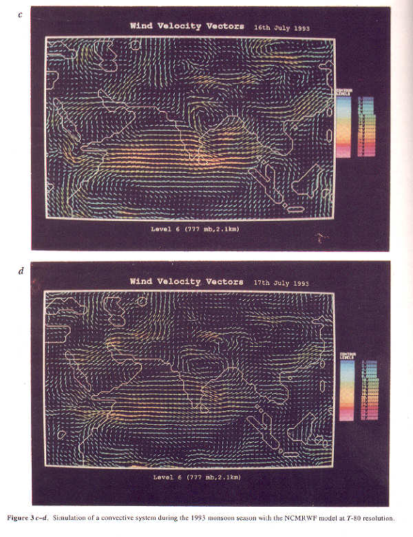
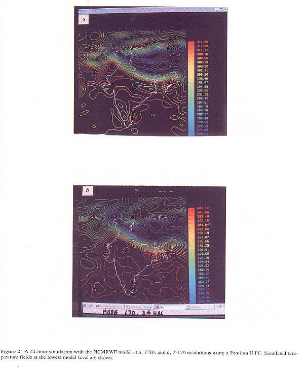
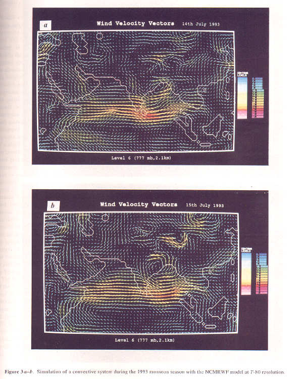
Figure 3 c–d.  Simulation of a convective system during the 1993 monsoon season with the NCMRWF model at T-80 resolution.

 

models can be executed even on PCs (Nanjundiah and Sinha¹⁸). A one-day simulation on a Pentium II PC takes about 45 min.

Specifically in the Indian context, massive parallel processing based on low-end processors such as Pentiums seems to be an attractive alternative.

Parallel computing of meteorological models

Parallel computing involves the decomposition of a single large task into smaller multiple tasks which can be carried out concurrently on a large number of processors. The most common method used for parallel processing is domain decomposition. For atmospheric models the global domain can be split into smaller sub-regions and the computations in each sub-region could be allocated to a processor. At required intervals during the temporal integration, data need to be communicated between processors. It should be borne in mind that interprocessor communication is an additional overhead for parallel computing and the time required for this should be a minimum for optimum throughput and maximum scalability, (i.e. increase in processing speeds with increasing number of processors). For most finite difference techniques data need to be communicated between neighbouring processors, and so a high degree of scalability is assured. However, spectral models need the communication to be global to transform variables from grid space to spectral space and vice-versa. This increases communication overheads and generally results in poorer scalability¹⁹. In most parallel implementations of spectral models, only the computations in grid space are parallelized. As the number of processors increases, the sequential component becomes more prominent leading to reduced scalability. However, with careful parallelization of the spectral component the scalability can be increased substantially. With proper stencils of communication, efficiencies greater than 90% can be achieved²⁰. Drake et al.¹⁷ have also shown that the spectral model CCM2 is also highly scalable on a variety of platforms. However, it should be noted that the computational flow in CCM2 is far more amenable to parallel computing than in the NCMRWF model used by Venkatesh et al.²⁰.

The NCMRWF model has been implemented in most of the leading parallel computing centres in India. It has been implemented on a variety of platforms at the National Aerospace Laboratories including a PC. In Figure 2 we show a typical forecast with the model at T-80 (standard resolution used at NCMRWF) and at T-170. We find that the higher resolution generates finer scale structures. In Figure 3, we show the evolution of a tropical depression over the Bay of Bengal as predicted by the model at a resolution of T-80. The movement of the depression is quite realistic.

Concluding remarks

Computational weather modelling has made rapid strides from the days of Charney et al.². Today, resolutions as fine as 50 km are possible with global models. In consonance with this, medium-range (5–10 days) predictions have improved dramatically in quality. However, the quality of the predictions in the tropics is still inferior to those in the mid-latitudes, being only about one-third of that in the northern hemisphere. Shukla²¹ attributes this to the differing nature of the convective disturbances while Krishnamurti²² suggests that the difference in data density is the primary cause. It must be noted that most major weather forecasting centres (such as ECMWF and NCEP) are in the mid-latitudes and their regions of interest are essentially the temperate regions. Thus improvement in the forecasts in these regions may not be surprising. It is necessary for Indian scientists to address problems relevant to tropical regions; furthermore, it is now being widely realized that further improvements at higher latitudes may become feasible only when tropical forecasts improve, because of global connections between different regions.

In the Indian context, the most important problems that need to be addressed are the following.

1. The prediction of the evolution and movement of cloud bands and the changes in associated rainfall. Predicting these will be of immense benefit to farmers and help them determine sowing and cropping patterns.
2. An accurate prediction of the movement of cyclones could result in improved disaster management.

 

It should be noted that realistic simulation of the seasonal mean patterns of the Indian monsoon with GCMs remains elusive²³. It has been shown that no GCM captures all the major features of the Indian monsoon.

Addressing these issues requires improvements to the model in terms of increased resolution and development of model physics and dynamics appropriate to the higher resolutions and the availability of good assimilated data. The computational resources have to be augmented
to generate predictions with such high resolution models in real time. Given the availability of expertise in
the fields of modelling and high performance computing in the country, achieving these objectives seems feasible.

 

---

1. Richardson, L. F., Weather Prediction by Numerical Process, Cambridge University Press (reprinted Dover, 1965), 1922,
   p. 236.
2. Charney, J., Fjortoft, R. and von Neumann, J., Tellus, 1950, 2, 237–254.
3. Kalnay, E., Sela, J., Campana, K., Basu, B. K., Schwarzkopf, M., Long, P., Kaplan, M. and Alpert J., Documentation of the research version of the NMC medium range forecast model,
   National Centres for Environmental Prediction, Washington DC, USA, 1988.
4. Holton, J., Introduction to Dynamic Meteorology, Academic Press, New York, 1972, p. 319.
5. Phillips, N. A., Mon. Weather Rev., 1959, 87, 333–345.
6. Lions, J., Temam, R. and Wang, S., Commun. Pure Appl. Math., 1997, L, 0707–0752.
7. Grell, G. A., Dudhia, J. and Stauffer, D. R., NCAR Tech. Note, NCAR/TN-398+IA, October, 1993.
8. Walko, R. L., Tremback, C. J. and Hertenstein, R. F. A., RAMS, The Regional Atmospheric Modeling System, Users Guide, Mission Research Corporation, Fort Collins, CO 80522, USA, 1995.
9. Orszag, S. A., J. Atmos. Sci., 1970, 27, 890–895.
10. Bourke, W., McAveney, B., Puri, K. and Thurling, R., Methods in Computational Physics (ed. Chang, J.), Academic Press, 1977, vol. 17, pp. 267–324.
11. Bandyopadhyay, S., Project Document, NAL PD FS9817,
    September, 1998.
12. Krishnamurti, T. N., Bedi, H. S. and Hardiker, V. M., An Introduction to Global Spectral Modelling, Oxford University Press, 1997, p. 237.
13. Krishnamurti, T. N. and Jha, B., Sadhana, 1998, 23, 653–684.
14. Asselin, R., Mon. Weather Rev., 1972, 100, 487–490.
15. Bhatia, R. C., Bushan, B. and Rao, V. R., Curr. Sci., 1999, 76, 1448–1450.
16. Dent, D. and Mozdzynski, G., Proceedings of the Seventh ECMWF Workshop on the Use of Parallel Processors in Meteorology (eds Hoffman, G. R. and Kreitz, N.), World Scientific, Singapore, 1996, pp. 36–51.
17. Drake, J., Foster, I., Michalakes, J., Toonen, B. and Worley, P., J. Parallel Comput, 1995, 21, 1571–1591.
18. Nanjundiah, R. S. and Sinha, U. N., Curr. Sci., 1999, 76, 1114–1116.
19. Basu, B. K., Curr. Sci., 1998, 74, 508–516.
20. Venkatesh, T. N., Rajalakshmy, S., Sarasamma, V. R. and Sinha, U. N., Curr. Sci., 1998, 75, 508–516.
21. Shukla, J., Adv. Geophys. B, 1985, 28, 87–122.
22. Krishnamurti, T. N., Annu. Rev. Fluid Mech., 1995, 27, 195–224.
23. Gadgil, S. and Sajani, S., Clim. Dyn., 1998, 14, 659–689.

ACKNOWLEDGEMENTS.  We thank NCMRWF for providing the initial datasets for the simulations.